Lesson 6 - Process Control Mechanisms

A PI controller combines the two terms for proportional and integral control that we encountered earlier.

The equation is as follows:

This is the sum of the two terms that we have just learned about. If we look at the figure below, we can see the control that PI gives us: 

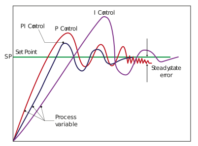
Figure: Combining proportional and integral control

As you can see, this results in a combination of the fast response of proportional control, along with the elimination of any steady state error, which is performed by the integral control.

In order to make these loops work correctly, we must understand the relative contributions of the two factors you can control with a PI controller. These two factors are known as the proportional gain and the integral time. These can be seen in the figure below:

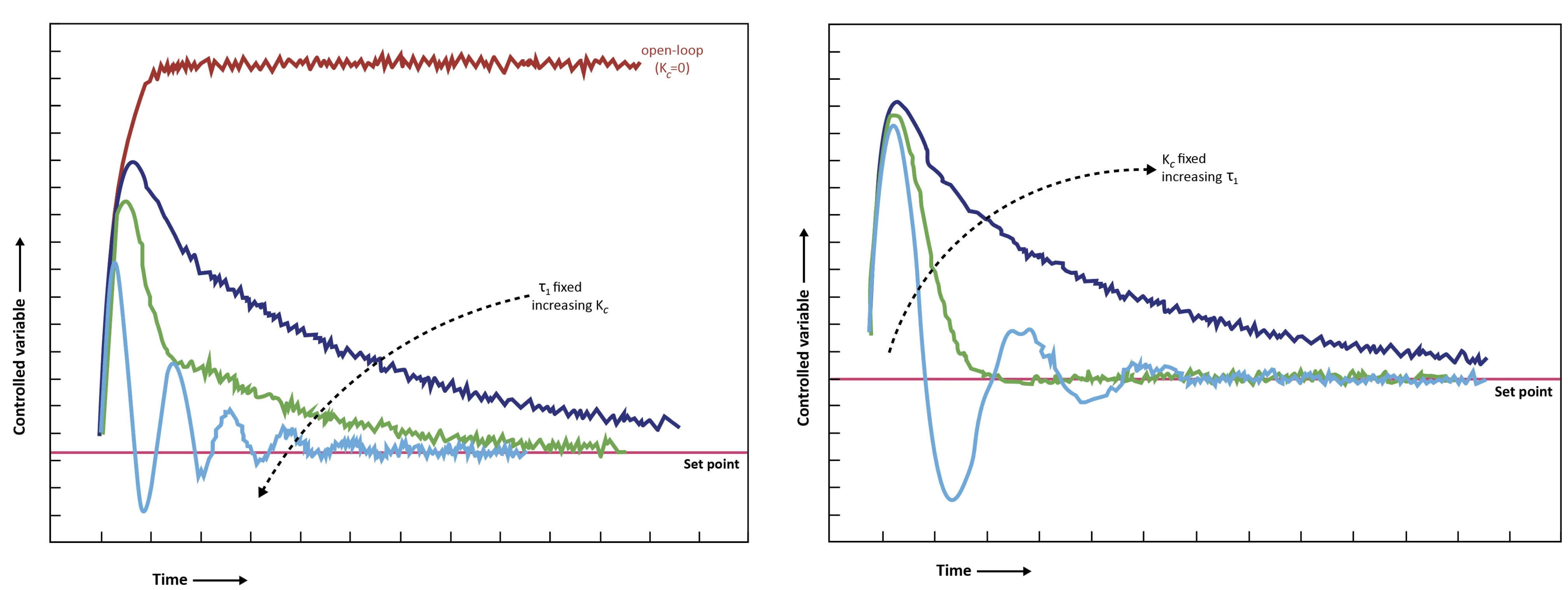
Figure: Relative effects of changing proportional gain and integral time

The first figure shows what happens if we increase the proportional gain (K_P) whilst keeping the integral time (T_I) constant. This has the effect of decreasing the offset and increasing oscillations.

The second figure shows what happens if we increase the integral time (T_I) whilst keeping the proportional gain (K_P) constant. This has the effect of decreasing the oscillations whilst increasing the offset.

So, what are the weaknesses of integral control?

• The process can start oscillating, as the integral term is still dwelling in the past and thus takes a while to catch up to the current situation.

• Integral control can lead to integral wind-up. If it is working correctly, the cumulative error should never be very large and should return to zero over time. Under certain conditions, the cumulative error keeps growing, which results in a delayed reaction when the setpoint changes.

The figure below shows integral wind-up in action, as well as how this can be overcome through using anti-wind-up protection:

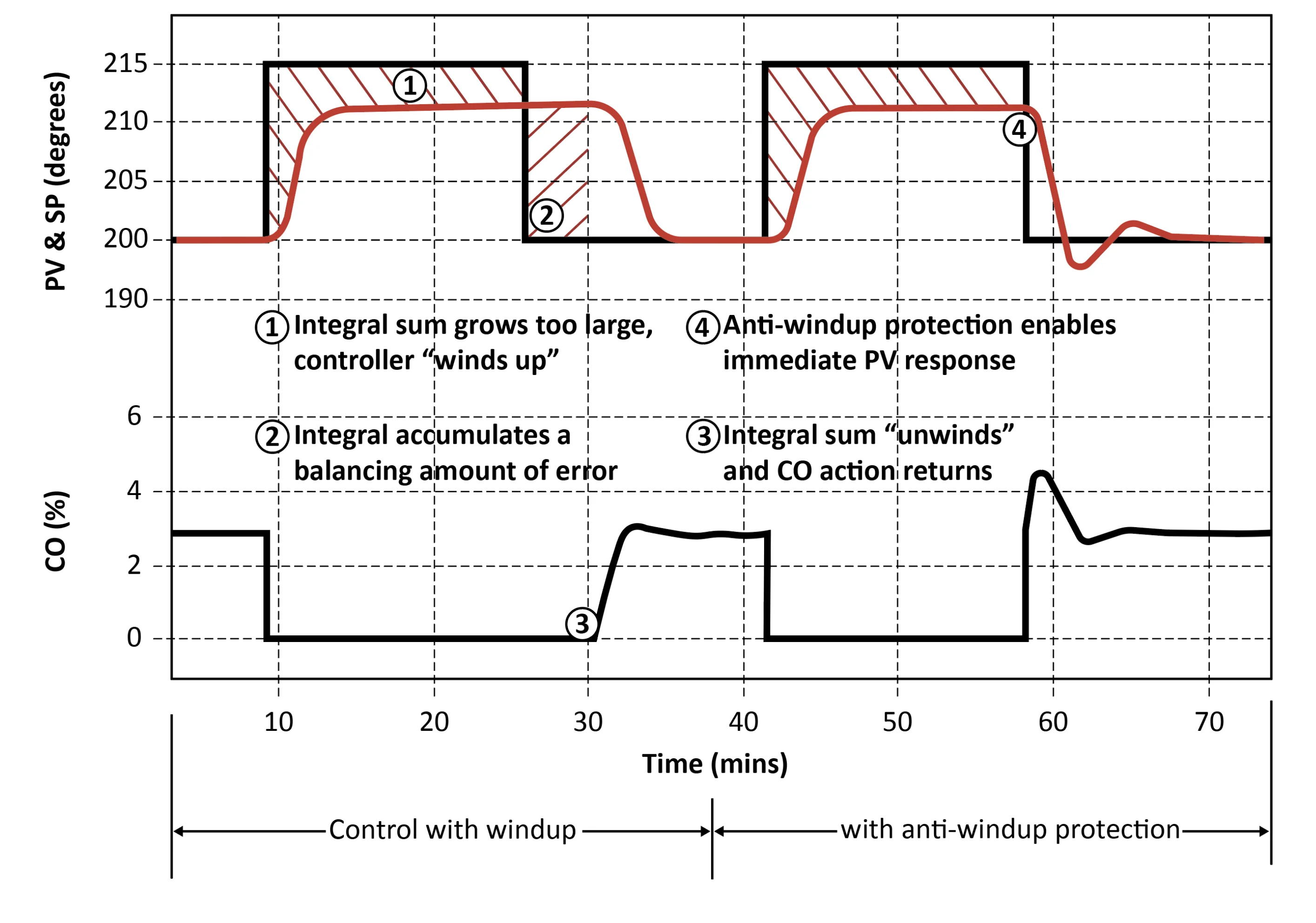
Figure: Integral wind-up and anti-wind-up protection

In the wind-up example above, the sudden change in setpoint creates a large integral error, which prevents the controller from opening until the integral sum has unwound. Some controllers have anti-wind-up protection built in.

Now we are ready to continue to the last term, which is derivative control. Whilst integral control was all about the past, derivative control is all about the future. The following figure represents this graphically:

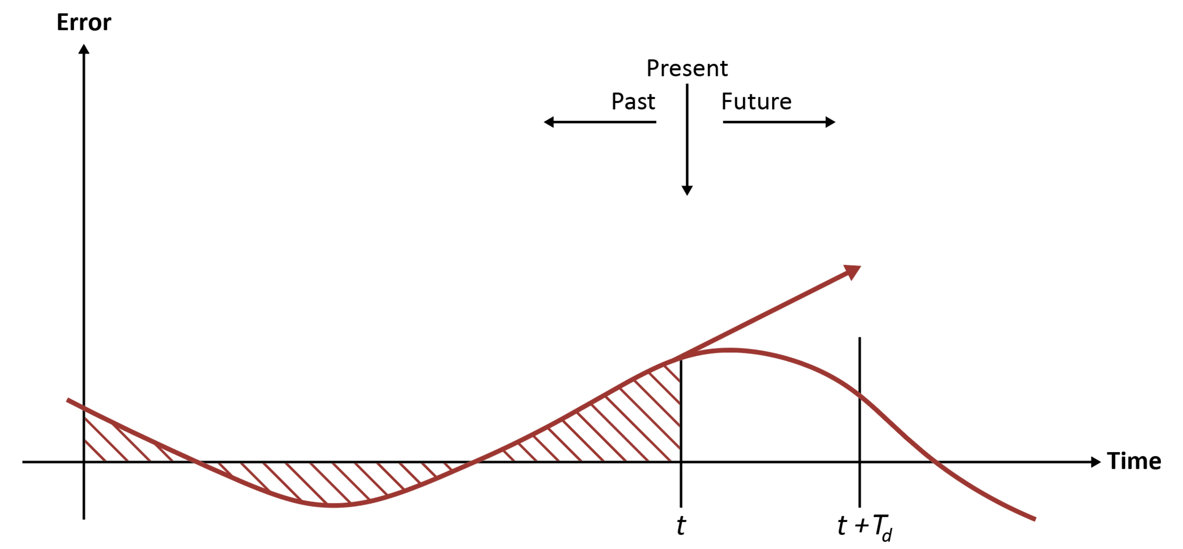
Figure: The focus of integral and derivative control