Lesson 6 - Process Control Mechanisms

Continuous controllers can adjust the controlled variable over a range. This allows them to potentially reach and maintain the process variable at the setpoint.

A common household example of a continuous controller is the temperature of your shower. By adjusting the hot water tap, you can get the temperature just right. If the temperature is too cold you can open it more, and if it is too hot you can close it more.

These are commonly referred to as control loops. As you can imagine, this is not an easy form of control to get right. Each process is different and the mechanism by which the controller adjusts the controlled variable will have to be different in each case.

Continuous controllers can have one, two, or three terms. These terms are:

• Proportional

• Integral

• Derivative

These can be used in various combinations, which we will explore later. Controllers that have all these terms are also called PID controllers.

Let us quickly look at some more terminology.

Process control terminology

We have already defined the setpoint as the desired value for the measured variable. Now let’s explain a few more terms.

Error is defined as the difference between the setpoint and the measured variable.

Duration is the length of time that an error exists.

Offset refers to when there is a sustained deviation between the measured variable and the setpoint. This can be seen as a persistent error. We will discuss this in greater detail when we cover proportional controllers later in this lesson.

Control loop descriptors

The following figure shows typical controller action:

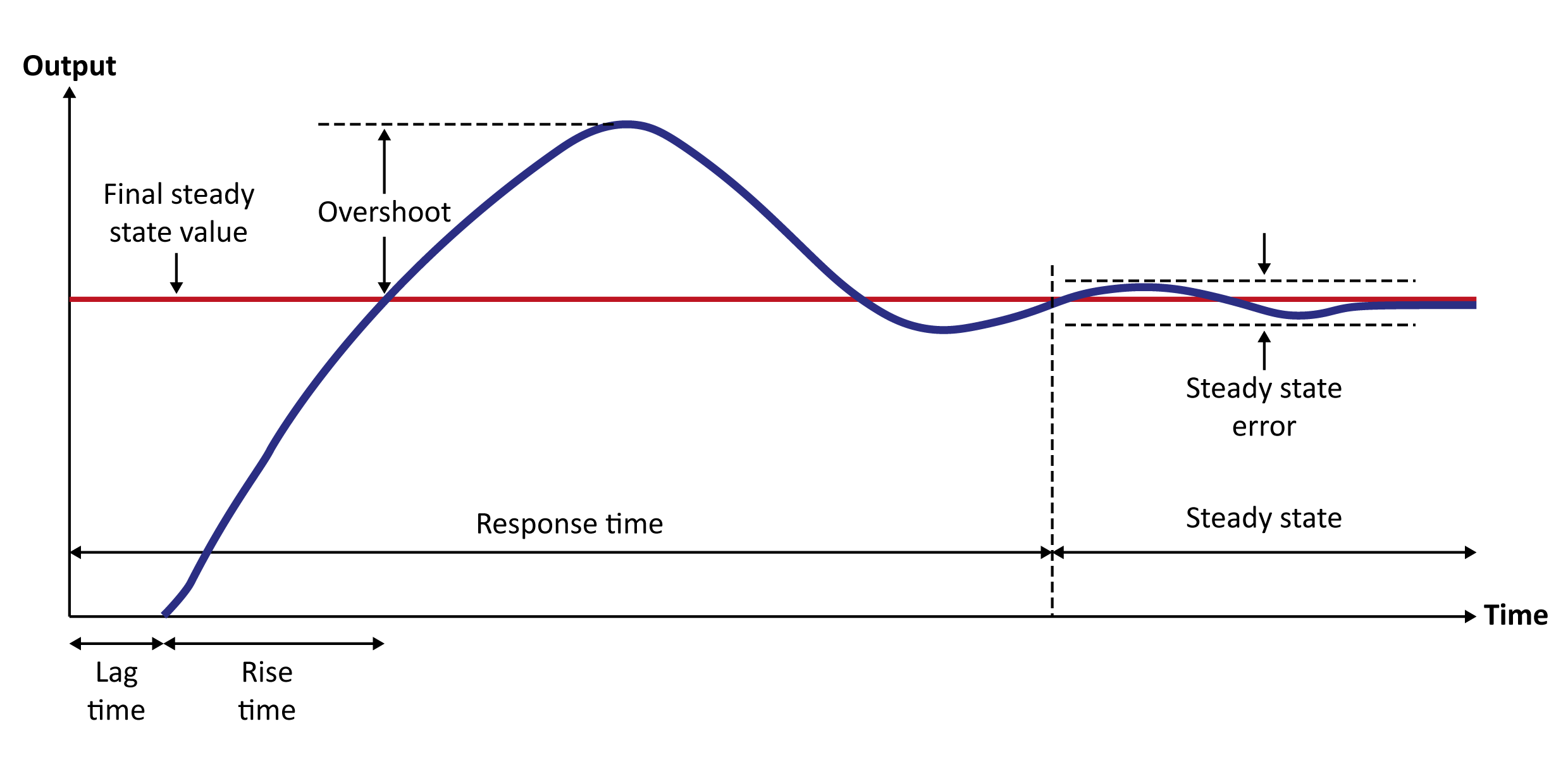
Figure: Typical controller action

Based on this, we can define some more key terms:

Overshoot is the ratio of the maximum amount by which the process variable exceeds the steady state value to the amount of the steady state. This is for the first attempt at control. Unlike offset, which is a persistent error, the overshoot is the maximum error that occurs the first time the controller attempts to bring the variable into control.

Rise time is the time required to reach the steady state value for the first time.

Response time is the time required for the response to settle out within a certain band of its new steady state value. Normally +/- 5% is the band. It is also referred to as settling time (in figure above).

Lag time is the time between the controller output changing and the process variable starting to change. It is also referred to as dead time (in figure above).

We can relate all these terms to what happens when we take a shower.

When standing under a shower, you open the tap. The first water coming out is freezing cold because of the cold water in the line between your water heater and the shower head. The time the water takes to start heating up is the lag time. You may then feel cold and open the hot water tap more.

The temperature then increases and becomes acceptable for the first time. This is an indication of the rise time.

If you overreacted to the cold you may have opened the hot tap too much and are now being scalded by boiling hot water. This is an indication of the overshoot.

You continue adjusting the tap and the water oscillates between too hot and too cold until you eventually reach a steady state and can enjoy your shower.

Controller tuning

What exactly do we want from a controller?

• A quick response to the error (you do not want to be freezing in that shower for a long time).

• To achieve a steady state or stable system.

• A steady state value close to the setpoint.

This is done by tuning the control loop. Tuning means that we change the controller terms until it acts as we want it to.

Direct acting and reverse acting controllers

Controllers can also be direct acting or reverse acting. A direct acting controller’s output will increase if the process variables’ values increase. Think of a valve for cooling water that enables cooling. The temperature of the water is the process variable and the valve is the controller. If the temperature rises, the cooling water valve will open more to bring the temperature down. A reverse acting controller’s output will decrease as the process variable increases. An example is a valve regulating gas flow to a burner. The temperature is the process variable and the regulating valve is the controller. If the temperature rises, the valve will close to bring the temperature down. The figure below shows these two operations:

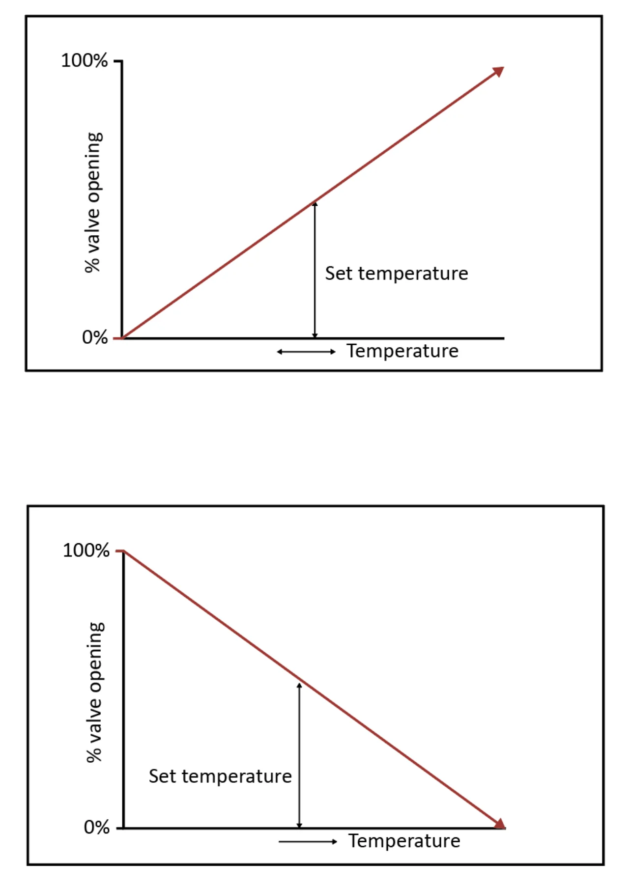
Figure: Direct acting and reverse acting controllers