Lesson 4 - Wort and Beer Analysis

All beer should be perfect and all lab analyses should be precise and accurate. However, there are variations at all stages of production and the results of all lab analyses vary to some extent. In this section we will discover what we need to do to develop robust specifications for our beer and analyses. First we look at how we term the reliability of our methods of analysis.

Repeatability r₉₅

Repeatability r₉₅, or within-lab variation, is a measure of the consistency of results from a method using:

• The same experimental tools

• The same analyst

• The same measuring instrument, used under the same conditions

• The same location

• Repetition over a short period of time

• The same objectives

The ‘95’ relates to the confidence level of the accuracy. If the same method, technician, and equipment were used for the same sample at the same time then the result produced would fall within the defined range 95% of the time or 19 times out of 20. The range is often given as the mean of the analyses results and then a figure which is the variation about the mean. For example, for method 19.9 in Analytica EBC for the measurement of calcium in beer by atomic absorption spectrophotometry, the mean figure is 22 mg/L and the r₉₅ is 3.7 mg/L.

Reproducibility R₉₅

Reproducibility R_95, also called between-lab variation, is a measure of the consistency of results from a method using:

• Different experimental tools

• A different analyst

• A different measuring instrument

• A different lab

• Testing at different times

Again, the ‘95’ relates to the confidence level so, in the above conditions, the result obtained from analysis on the same sample would be within the stated range 19 times out of 20. R₉₅ is virtually always higher than r₉₅. With our example of calcium levels the R₉₅ is 14.6 mg/L. R₉₅ figures are established by EBC, ASBC, and MEBAK with the use of a number of large brewery or independent analytical labs.  

Why set specifications?

Specifications enable us to consistently meet the needs and expectations of our customers. We need to set specifications to give us a target to aim for and a realistic range of values over which variation is acceptable to the customer. The target and the range must be achievable within the variation of the process when it is operating in control. The range must also encompass the R₉₅ for the analytical process. There would be little point in setting a spec where analytical errors consistently led to good product being classed as out of spec. So how do we set these ranges? 

Specification ranges (tolerances)

As we saw earlier, R₉₅ are available for most methods so we can use these to set a minimum range or band width. We can also use data from the process using statistical process control (SPC). We will start with this SPC approach.

Band width using SPC

As we saw in the Quality Assurance and Quality Management lesson, data within a process are usually assumed to be distributed normally about the mean. The spread of data is represented by the standard deviation, σ. For each σ level that we move away from the mean, the greater amount of data is included. The figure below shows the percentage of data which is included, and so variation explained, for each standard deviation away from the mean.

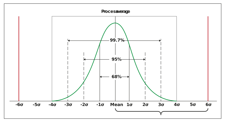
Figure: Normal distribution and standard deviations 

To ensure we capture all possible variation, we use 6 x σ and beyond as the band width for our specification. The specification band width is the interval between upper A2 and lower A1 limits. The ratio of the specification band width to 6 x σ is termed the process capability (Cp) and is shown in equation 1 below.

Equation 1:

The table below shows the rate of rejects to be expected for a range of process capabilities. 

Table:  Rejects based on process capability 

The goal is to have a Cp value that is as high as possible, but at least 2 is usually recommended for setting a specification band width. Let us work through an example:

We have a beer with a target colour of 10 EBC. We have undertaken analysis of samples of the beer from BBT over two months and calculated the variance of colour to be 0.0576 EBC.  From this we can calculate σ.

To work out our band width we rearrange Equation 1 above and use 2 as our process capability to get:

This is the band width so we need to divide it by 2 to get the figure by which it varies from the target value 10 EBC. The specification is therefore: 

In the next method we use R_95­  and SPC principles to set the band width.

A beer has a colour target value 10 EBC and R₉₅ is 0.68 EBC.

R₉₅ has been established in ISO 5725 to be 2.8 x standard deviation (where standard deviation is an estimate of the true standard deviation σ). So, we need to divide R₉₅ by 2.8 to get the standard deviation.  

And to work out our band width we rearrange equation 1 above and use 2 as our process capability to get: 

This is the band width so we need to divide it by 2 to get the figure by which it varies from the target value 10 EBC. The specification is therefore:

Band width using ISO 4259

Before we look at using the ISO 4259 standard it is important to note that it relates to precision of measurement methods and results for petroleum and related products. This means samples it deals with are likely to be more homogeneous than brewery samples so will not have the same problems with sampling. 

ISO 4259 states that specification limits should be expressed as 'not less than' or 'not greater than'.

Limits may be either:

• A double limit, upper and lower (colour or bitterness for example)

• A single limit, upper or lower (upper for ATNC or lower for friability, for example)

The value chosen for the specification limit should take into account R₉₅ for the method.  For a double limit the specified range should not be less than 4 x R₉₅ or: 

Using our 10 EBC target above, the recommended specification band width would be:

So, as above, we divide by 2 to get the difference of specification limits to the target:

So, our specification is not less than 8.64 EBC and not greater than 11.36 EBC.

For specifications where this is a single limit, there will often be another physical limit, 0 or 100% for example. In these cases, the limits should be constructed so that they are greater than or equal to 2 x R₉₅ from the physical boundary.

Simple probability calculations – variance, standard deviations, and the z-score

We have encountered normal distributions and standard deviations a number of times throughout the Quality Management unit. Now we are going to discover how to calculate it. This is the formula for the standard deviation, or s, where X = the individual result, xbar = the mean result, and n = number of results:

We will work through this in an example. We have the results from multiple spectrophotometric analyses of colour for a brand of beer in BBT in the last few months and have selected a sample of five results to use for our calculation. Here are the results in the sample.