Lesson 10 - Carbon Dioxide Recovery Technology

In the same way that a good brewer should be able to estimate ethanol yields from wort, we should be able to do the same thing for CO₂ (estimate its yield from fermentation). To do this, we need to return to the Gay-Lussac fermentation equation (discussed in the Gases Unit) and work with molecular masses, as was done previously in our consideration of gas laws in that unit.

The Gay-Lussac equation tells us that for every kmol of glucose (C₆H₁₂O₆) fermented, 2 kmol of CO₂ are produced.

The respective molecular masses are (6 x 12 + 12 x 1 + 6 x 16 =) 180 kg/kmol for glucose, and (12 + 2 x 16 =) 44 kg/kmol for CO₂, hence the yield of CO₂ is:

We can assume that 1 kg of glucose is equivalent to 1 kg of sucrose (this is not strictly correct as there is a hydrolysis reaction of sucrose to glucose to account for but let us ignore this for the moment).

It should be noted that this would be an idealised amount of CO₂ produced during fermentation and it does not account for any carbon utilisation towards biomass or other fermentation products nor other losses (more on these later in the lesson). In addition, not all of this quantity of CO₂ would leave the fermented wort and be available for recovery. Some would stay in solution, which varies considerably depending on the size of the fermenter (mainly related to wort depth), the altitude of the brewery, and the approach to fermentation management, (e.g. pressure fermentations). Therefore, it can be difficult to estimate the remaining dissolved quantity.

If we look in a little more detail at a fermentation (or attenuation) profile (see below), we can appreciate the decline in the real extract from the original extract (OE) value to the end-of-fermentation (EOF) value. The fermentable range (OE – EOF), can be directly translated to both the quantity of alcohol produced (which we may be more familiar with), as well as the quantity of CO₂ produced. So, all other things being equal, the fermentable range of a wort/beer will directly affect the quantity of CO₂ produced.

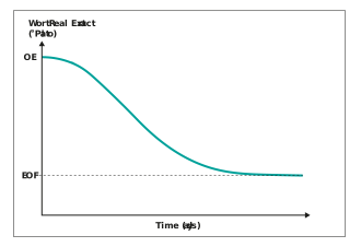
Figure: A fermentation attenuation profile

The yield figure, together with fermentation range, can be used as a basis against which collected and lost quantities of CO₂ can be normalised against.

Example:

A brew of 600hl collected volume had an original extract value of 15 °P (density 1061.1 kg/m³). Following the completion of fermentation, the end-of-fermentation real extract was 3 °P (density 1011.7 kg/m³) Determine the following:

a)    The idealised total quantity of CO₂ produced during fermentation.

b)    If 2,000 kg of CO₂ was purified and liquefied from this fermenter, what would be the percentage collection efficiency, using the figure in point a) above as a basis?

a) At an OG of 15°P, wort has a density of 1061.1 kg/m³, so 1m³ of wort weighs 1061.1 kg

15°P wort is 15% w/w sugar so 1m³ contains 15/100 x 1061.1 = 159.165 kg of sugar

At an FG (real attenuation) of 3°P, wort density is 1011.7 kg/m³ so 1m³ of wort weighs 1011.7 kg

3°P wort is 3% w/w sugar so 1m³ contains 3/100 x 1011.7 = 30.351 kg of sugar

So sugar fermented is 159.165 – 30.351 = 128.814 kg

Since for every 1kg of sugar fermented we get 0.49 kg of CO₂, the CO₂ evolved = 128.814 x 0.49 = 63.12 kg

If 1m³ of wort at 15 yields 63.12 kg, 60 m³ (600 hL) would yield 60 x 63.12 = 3787.13 kg

b) If 2,000 kg of CO₂ was purified and collected, then the percentage collection efficiency would be given as:

Single fermenter CO₂ production rate

We have just described the ideal CO₂ yield (kg per °P per kg of sugar fermented) and the use of a fermentation (or attenuation) profile to utilise the fermentable range (OE – EOF RE) in determining the total quantity of CO₂ which we can ideally expect throughout a fermentation. But what about the rate of CO₂ production from a single fermenter? Would we expect this to be a constant or would it vary during a fermentation? Consideration of the attenuation profile together with the CO₂ yield figure, will answer these questions.

Let us remind ourselves what we mean by fermentation rate. The rate would be the change of wort gravity with time. This can also be thought of as the gradient (∆y/∆x) of the attenuation curve at any point in time. This is shown in the figure below, where the rates of fermentation are indicated at the start, middle and end of fermentation.

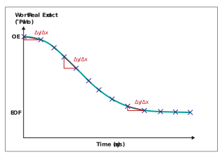
Figure: A fermentation attenuation profile showing daily fermentation rates at the start, middle and end of fermentation

We can see that the fermentation rate – the gradient ∆y/∆x – is low at the start, increases in the middle of fermentation and reduces near the end. Such values of fermentation rate can be determined from the change in daily wort gravities and plotted, as shown in the figure below.

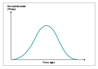
Figure: The fermentation rate over the course of a fermentation

In the fermentation rate figure above, you can see that fermentation rate is expressed, in this example, as the number of Plato fermented out per day and this rate is zero at the start of fermentation and thereafter it rises to a maximum, during mid-fermentation, and then drops off to zero at the end of fermentation. Such fermentation rate information can be combined with the CO₂ yield figure, we introduced earlier, to produce a CO₂ production rate profile, as shown below.

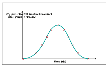
Figure: The daily CO₂ production rate over the course of a fermentation

The CO₂ production rate profile has the same shape as the fermentation rate curve, starting at zero and rising to a maximum and then dropping off to zero as the fermentation rate slows down.

It is clear that the rate of CO₂ produced is not constant; it builds and then dissipates significantly during fermentation. It would be very rare for a single fermenter to have a CO₂ recovery plant associated with it. We can now consider the more common situation within a fermentation block, i.e. multiple fermenters, and how the presence of multiple fermenters affects the rate of CO₂ produced by the room.