
Lesson 6 - Sensory Analysis
This lesson deals with the sensory analysis of beer. It details how to set up the elements of a sensory panel, such as panel selection, training, and the design of the sensory facilities, and then covers how to run the panel and collect the results. It discusses the various types of sensory test and their benefits before going on to cover the use of statistics to convert sensory data into information about the sensory quality of beer. Finally, it looks at the presentation of results from sensory tests and lists key flavour compounds in beer.
Presentation of Results
Now that our sensory data have been converted into a form we can trust (within the limits of statistical significance) the next step is to communicate the findings to those interested.
For routine sensory data aimed at production, a table of results will be all that is required to convey the message, but in many circumstances we will need to provide a written report of the findings of the analyses. This report should be in a form appropriate for the reader. For example, key flavour terms would need to be defined if the readers are not technically trained, or commercially significant elements emphasised for management. The summary of results should not be more than 110 words and it should set out:
-
The objective of the analysis
-
What was done
-
The results
-
What can be concluded
Text should be supported with the appropriate tables, charts, and graphs. We will now discuss each of these.
Tables
The strength and the weakness of a table are the same thing, namely it can provide a great deal of information. Presenting a table of all the data from a flavour profiling exercise would be bewildering to readers and pointless. Simple summary tables where key points are emphasised with different colours or degrees of boldness are more instructive and can convey information less confusingly than elaborate graphs.
Histogram
Histograms are useful for flavour profile data presentation. They allow comparisons of attribute intensities between samples. Introduction of a second scale allows other data (such as process parameters) to be added to the histogram to enable a comparison. An example of a histogram comparing three different IPAs across a range of attributes is given below.
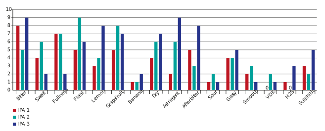
Figure: Histogram comparing three samples of IPA
Spider diagrams
Spider diagrams are the most commonly used graph to present the data from a descriptive analysis test. They give the overall flavour a shape which enables a clear comparison of different beers when they are plotted together. Below is the example of a spider diagram comparing the same three IPAs.
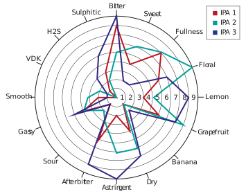
Figure: Spider diagram of three IPAs
We have now undertaken the complete journey from selecting our panel, through selecting and undertaking our tests, to publishing our results clearly and effectively. In the final section of this lesson we will discover the compounds that are responsible for some of the aromas and tastes we experience in beer.