Lesson 6 - Sensory Analysis

We now have our sensory data but we need it in a form that we are confident is correct and that clearly and accurately displays a true picture of how the beer tastes. This section shows us how we check the data using statistics and the next section then looks at how we display and report the results.

Even the best statistical package, applied brilliantly to a set of data, will not make sense of results that come from a badly designed test. It is essential to ensure that the purpose of the test is well defined and understood, the correct test for the purpose is applied, and sufficient data from a sufficient number of panellists are obtained.

We now cover the simpler principles of statistical analysis and work through a general explanation of the more complex ones. Increasingly, computers carry out most of the statistical processes.

In the introduction we learned that the equipment we use (humans) is prone to error. Even the most highly trained and experienced panels will give different results on different days. So, as well as variation in any beer, there will be variation in the panel’s perception. In descriptive tests you can evaluate this variation simply by having the panel taste the same beer for several days in a row and calculating the mean and standard deviation of scores for each attribute.

Confidence and significance

Because we are not dealing with perfect machines or definitive outcomes, we tend to report results with confidence levels and significance levels. Confidence levels express how likely it is that the results have not occurred by chance. The most commonly used confidence level is 95% which is the equivalent of a 5% significance. This equates to 95 scores in 100 being correct. We use confidence and significance levels when reporting the results from difference testing. It is important to note that even a confidence level of 99.9% does not mean we have a definitive answer. For example, if 7 in 10 assessors correctly identified a difference in a Triangle test this would give us a confidence level of 95%. If we repeated the test with 30 people and 21 correctly identified the difference, the confidence level would be 99.9% even though the proportion of the assessors who were correct was the same. Increasing the number of assessors just allows us to conclude that the probability of getting the correct outcome by chance is lower.

Analysis of variance (ANOVA)

ANOVA is used for the data from descriptive tests as a means to make sense of the vast array of numbers generated. We saw earlier that flavour profiling is carried out by eight panellists assessing around 50 attributes, so each profile will consist of 400 scores. ANOVA is basically an extension of the use of simple statistics (like means and standard deviations) and tests to determine if differences are significant. ANOVA is used to assess the variability of the scores given for repeated analyses of a given beer relative to the variability between the assessors.

In ANOVA we calculate the F-ratio, which is an index of the variability in the data. F-ratios are calculated for variations between the beers and between the assessors.

Principal component analysis (PCA)

PCA is a method of identifying patterns of difference or similarity in data between beer flavour profiles. The analysis is very complex and undertaken by a computer; this section provides just a brief overview.

PCA seeks to explain variability of the data by grouping together attributes. The first principal component will be identified and the amount of variability that it explains calculated. The analysis will then move on to the next principal component until all the variation is explained. The majority of the variation will often be explained by the first two or three principal components.

The results of PCA are displayed on a graph. The graph shows the position of the original beer as a single point. Points which are close together are more similar, those further apart less so. Attributes are plotted as loadings on the outside of the graph and beers will appear closest to the attributes that are present in them. The figure below shows a PCA graph for standard lagers from four plants.

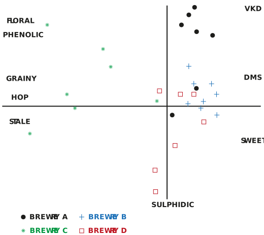
Figure: PCA plot for standard lagers from four plants

The plot shows that lagers from plants A, B, and D are generally well matched while lagers from plant C differ to the others by being hoppier, staler, and more grainy.

PCA is a good tool for comparing the data from large numbers of different beers, with more than 20 easily practicable. It can also be useful for comparing differences between commercial beers in the same style. Doing this and comparing the results to sales data can help to identify which flavour attributes are common to successful brands which can give a prototype for new product development. PCA can also be used to examine flavour-matching across sites that make the same brands. If the beers from one site are found to form a discrete group on a PCA plot it will show they are not matched.

Factor analysis

Factor analysis is used to establish if a high correlation in the data from a group of variables could be due to a common factor, for example if the levels of malty, fullness, and sweetness for a beer were associated with a process parameter like mash temperature. Factor analysis seeks to link key flavour attributes with key causal factors. It is related to PCA and there is some debate between statisticians about differences between the two approaches.

So, we have made some sense of our data. However, it is not quite ready to present to our stakeholders. The next section deals with how we communicate our findings effectively.