
Lesson 8 - Control of Fluid Flow 1
This lesson will consider two main classifications of pumps: centrifugal and positive displacement. These will be introduced together, with aspects of their design and operation. The lesson will also pull together various fluid mechanics concepts from previous lessons, such as the Darcy-Weisbach equation and the use of loss-coefficient to calculate pressure drops in pipe systems. It will use this information to then size pumps for particular pipe systems.
Matching Pump Characteristics to Pumping Duty
There are two methods to consider which can assist us in matching a pumping duty to a pump, or vice versa. Both methods will be explained as graphical methods. The first one deals with where a pairing of pipe system flow rate pressure-drop data points sit on a pump curve. The second one deals with a more extensive relationship for the pipe system flow rate pressure drop and how it matches a pump curve.
Pipe system operating point matched with a pump curve
In this method, we simply consider what we want the pump to provide the pipe system with. That is, what flow rate (capacity) and pressure (total head) do we wish the pump to supply to our pipe system? For the purposes of this method, we will assume that the flow rate, pipeline geometry, and layout are known. We will assume that we have calculated the pipeline pressure drop using the methods we have studied previously, e.g. the Darcy-Weisbach equation, and the loss coefficients for the various line fittings, such that we know the required flow rate QR and total head ∆Ps the pump has to supply.
If we are considering utilising one of a series of pumps represented by the following pump curves shown below, we would simply plot QR and ∆Ps on the pump curves. From the figure below we can see the pipeline requirement (QR, ∆Ps) lies on the operating curve of pump model #2 which suggests that pump #2 would be able to provide the required capacity and total head to match the pipe system requirement. However this is a simplified view, and there may be valid reasons for selecting the next, larger size of pump, #3. This depends on our level of confidence in pipe system design (i.e. desired contingency) , or allowance for potential future increases in flow or head. Generally, we would not select a pump whose curve lies below the desired operating point!
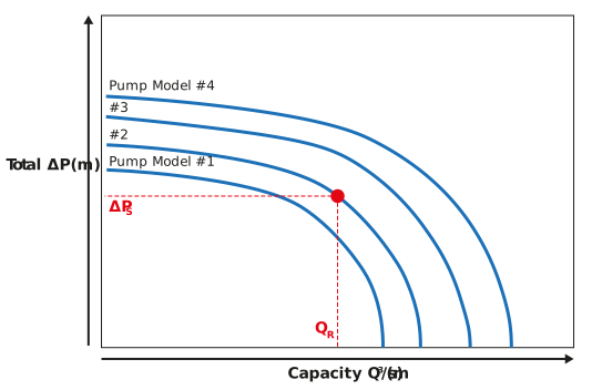
Figure: A series of capacity-total head pump curves and a pipe operating point
Pipe system characteristic curve matched with a pump curve
This method is an extension to the previous method in that it uses flow rate (capacity) and pressure (total head) data that we wish the pump to supply to our pipe system. However, it extends the consideration of only one data point, to rather a consideration of a set of flow rate pressure-drop data.
As above, we will assume that the flow rate, pipeline geometry and layout are known and that we have calculated the pipeline pressure drop variation with flow rate using the methods we have studied previously, e.g. the Darcy-Weisbach equation and the loss coefficients for the various line fittings. Let us say, for the sake of argument, that we have a dataset consisting of five pairs of data which we could plot on a pump curve as shown below.
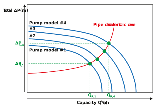
Figure: A series of capacity-total head pump curves and a pipe operating curve
If we drew a curve through these five pairs of data (indicated as x), as shown above, to form a pipe characteristic curve we can see that at the various points, where the pipe characteristic curve intersects with the four pump curves, that each pump model would operate with a different capacity and total head. Take pump models #1 and #4 as extremes, we can see that they would have operating points of (QR,1, ∆PS,1) and (QR,4, ∆PS,4). In practice, one would compare the required capacity and total head with these four operating points and select a pump model accordingly.
Let us look at a worked example to understand this concept of pump and pipe matching further.
A centrifugal pump has the following operating characteristics:| Capacity (m³/s) |
0 |
0.005 |
0.01 |
0.015 |
0.02 |
0.025 |
0.03 |
|
Total head (m) |
14.2 |
13.6 |
12.9 |
11.8 |
10.7 |
9.0 |
6.4 |
A pipeline is fitted to the discharge side of the pump and the pipeline has the following characteristics:
|
Capacity (m³/s) |
0 |
0.005 |
0.01 |
0.015 |
0.02 |
0.025 |
0.03 |
|
Head loss (m) |
0 |
0.25 |
1.02 |
2.29 |
4.08 |
6.37 |
9.17 |
By assuming that the suction head on the pump is zero, determine the operating point of the pump and state the associated capacity and discharge pressure at that point?
We can deal with this problem, one stage at a time. First, let us plot the pump curve data. This is shown below.
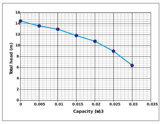
We should remind ourselves that this data and plot represents the total head, across the pump between suction and discharge that the pump can generate at various values of capacity.
If we now separately plot the pipe characteristic data below:
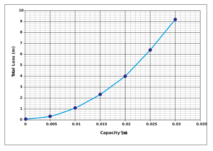
Again, let us remind ourselves, what this data and curve represent. It is the head loss across a pipe as a function of flow rate (or capacity). Typically, this data would come from repeat applications of the Darcy-Weisbach equation and/or loss coefficients, which we have covered in earlier lessons.
In order to find the operating point of the pump, we simply overlay the pump curve with the pipe characteristic curve and note where the curves intersect. This is plotted below.
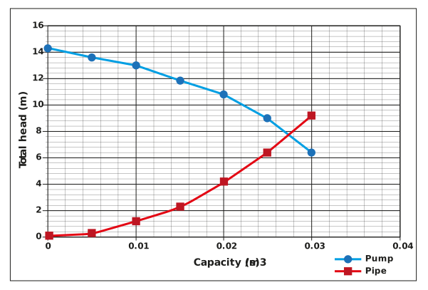
The operating point – the point of intersection of the pump curve and pipe characteristic curve – is at a capacity of 0.028 m3/s and a total head of 7.6 m.
We have covered a lot of detail on matching pumps to pipe systems and determining the resulting flow rate (capacity) and total head supplied. We can finish off our consideration of pumps with some thoughts of how to control pumps when starting them and how to control the pump performance using a variable speed drive.