
Lesson 8 - Control of Fluid Flow 1
This lesson will consider two main classifications of pumps: centrifugal and positive displacement. These will be introduced together, with aspects of their design and operation. The lesson will also pull together various fluid mechanics concepts from previous lessons, such as the Darcy-Weisbach equation and the use of loss-coefficient to calculate pressure drops in pipe systems. It will use this information to then size pumps for particular pipe systems.
Centrifugal Pump Operating Characteristics
Centrifugal pumps are often considered the workhorses of the brewing industry, for reasons we have previously discussed, but their performance and the interpretation of performance specifications is also often misunderstood. Let us look at these specifications, how they can vary, and how we can interpret them correctly to help towards choosing a pump suitable for a particular task.
The pump curve
The simplest and most effective way to consider the operating characteristics of a pump is in a graphical form, known colloquially as a ‘pump curve’. A typical pump curve is shown in the figure below.
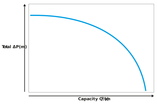
Figure: A capacity-total head pump curve
In the pump curve, we can see that:
-
Neither capacity nor total head are constant; in fact, they are strongly interrelated and inversely related. We will see later in this lesson that we cannot determine what capacity and total head a centrifugal pump will deliver without also considering the piping system it is intended to supply.
-
At the point where capacity is zero, i.e. when the flow rate is zero which could be achieved by closing off a valve on the discharge side of the pump, the total head is at a maximum. This condition is called ‘dead-ending’ a pump.
-
The point where the pump supplies its maximum capacity is when the total head on the pump is zero. This condition is termed the ‘zero-head’ flow rate and can be approached in practice when a pump is completely disconnected from a delivery pipeline, and a zero suction head is placed on it.
A centrifugal pump operates under a compromise between capacity and total head. It can deliver elevated levels of capacity but not whilst developing a large total head, or conversely, it can deliver a large total head but with a reduced capacity.
You will remember from our definition of pumping power, that it is the product of total head and capacity. Therefore, from the pump curve, we can easily plot pumping power against capacity. This is shown in the figure below.
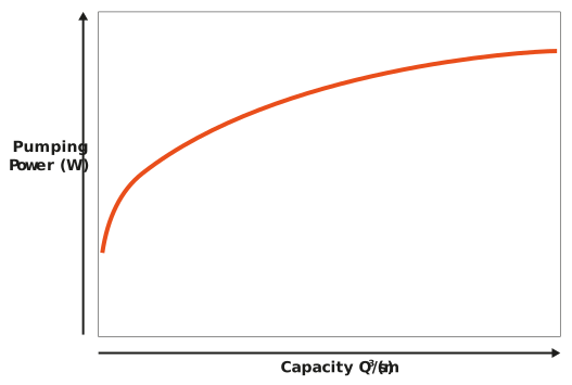
Figure: A capacity-pumping power pump curve
We can see that as the capacity of the pump increases the pumping power increases too.
Finally, we can consider how efficiency varies with capacity in the figure below.
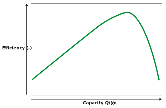
Figure: A capacity-efficiency pump curve
As we mentioned previously, efficiency can vary significantly with pump capacity. Furthermore, we can see that efficiency has a maximum part way along the capacity range for a pump (this is termed a local maximum condition).