Lesson 4 - Gas Transfer

At the very beginning of the section on saturation and Henry’s law, we considered a plot of dissolved gas concentration against time, to introduce the steady-state concept of saturation. Many gas transfer processes can take a considerable time to reach equilibrium, a period which we may not have time for in our busy lives! Let’s have a look at which parameters influence the speed (or rate) of gas transfer, so that we know how we can influence the speed of gas transfer to suit our level of patience!

Previously, we considered Henry’s law and how, under equilibrium conditions, a gas will exert a partial pressure above the liquid proportional to its molar fraction. However, if the gas is at a pressure above its equilibrium pressure, then gas will pass from the gas phase (headspace) into the liquid phase. This is the concept of forced carbonation in which, for example, we apply an elevated CO₂ headspace pressure in a keg to ‘force’ gas to dissolve into the beer. We considered such a situation previously, and the behaviour is represented in the figure below.

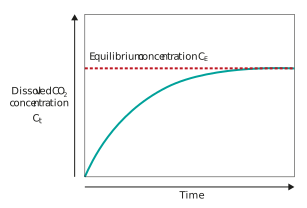
Figure: Plot of dissolved CO₂ concentration against time

The rate (or speed) of the dissolution process is given by the gradient of the curve at any point on the curve i.e. where the concentration C_t is a function of time t. We should, however, note that this representation (and the equation below from which it originates) applies to the special case of non-forced/non-agitated conditions on both the gas and liquid side.

Let’s look at this equation to understand each term (we won’t consider each term in order so stay with it):

• C_t – this is the dissolved gas concentration at any time t.

• dC_t/dt – is the rate (or speed) of change of the dissolved gas concentration. You can also think of this as the gradient of the graph. Clearly, this gradient is not constant – it starts off quite high (the curve is initially steep) and then it reduces (the curve flattens out as equilibrium is approached).

• C_E – is the equilibrium (or saturated) dissolved gas concentration, for a constant gas phase partial pressure.

• A – is the area between the gas and liquid phases. An example of A in a bottle of beer would be the circular area of the top of the beer in the neck of the bottle, as this is the interface between the beer below and the gas above in the headspace. Any transfer of gas into or out of the beer from the headspace would have to be transferred across this area. Alternatively, if we were bubbling gas through the liquid – like an aerator in a fish tank – A would be the total surface area of the stream of bubbles.

• V – is the liquid volume. Easy enough to understand, it is the volume of beer in the bottle in the example above.

• The grouped parameter A/V is referred to as the specific surface area (and generally denoted ‘a’). It is the surface area to volume ratio and is quite a useful parameter to consider. A large interfacial area A to a small volume V, will give a large A/V. We will look at it in a little more detail soon.

• k_L – this is termed the ‘mass (gas) transfer coefficient’. It is quite an abstract concept, but you can think of it as a numerical value which represents how intensely the gas and liquid phases are brought together or in contact. So, in the case of the headspace in the beer bottle above, where the intensity of contact would be very low, the mass transfer coefficient would also be low. However, in the fish tank example, a stream of bubbles would be considerably more intense, so the k_L value would be greater. You will see later how we can engineer systems to influence k_L.

So, let’s consider three differing gas transfer situations and we’ll apply the above rate equation to determine whether these situations result in a high or a low rate of gas transfer:

Situation 1. Consider you wish to carbonate 50 L of beer, which you have carefully crafted at home, using 50 L (working volume) kegs and a pressurised CO₂ gas supply which you can connect to the headspace of the kegs. Keeping all other parameters constant, with the options of carbonating all 50 L in one keg or instead splitting the beer into 25 L each in two separate kegs, which option would carbonate more quickly (i.e. which option would give the higher rate of gas transfer)?

Situation 2. Regardless of the volume of beer you chose to carbonate, and leaving all other parameters constant, consider which of these options would carbonate the beer more quickly if you connected the CO₂:

• Leaving the keg untouched

• Vigorously shaking the keg regularly to swirl the contents around

Situation 3. Irrespective of your choices to the first two parts above, if in your choice of CO₂ gas pressure you used the equilibrium gas pressure equivalent to the final required v/v of CO₂, or one which was 50% higher, which one would carbonate more quickly?

Give yourself 5-10 min to think about this, and then click ‘Next’ to continue with this lesson.