Lesson 4 - Principles of Fluid Mechanics 2

If we take our pipe full of fluid from the previous description of laminar flow, and substantially increase the flow rate, and therefore the flow velocity so that the Reynolds number exceeds 4,000, we would see a much different flow from laminar. Instead of the smooth-flowing, well-ordered laminar flow, the flow would be highly chaotic and crowded with many eddies of different sizes present (you can think of an eddy as a rotational flow, a little like a very small tornado). We term this kind of flow regime as a turbulent flow (turbulent is derived from the Latin turbulentus meaning ‘crowd’).

Measuring and plotting the velocity profile of turbulent flow can be difficult. There can be so much chaos and variation of local velocities, that no one value of velocity measured in one position would appear representative. However, over time, we can average such variations in local velocity, to produce a plot such as the one below.

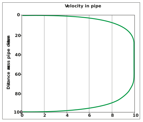
Figure: Time-averaged velocity profile of turbulent flow across a pipe

Things to take note of in this profile include the following:

• The velocity of the fluid next to the wall (at 0 and 100 mm across the pipe) approaches zero (remember this was the same for laminar flow).

• The velocity increases very rapidly as we move away from the wall and reaches near its maximum value a short distance from the pipe wall.

• The maximum velocity is at the centreline of the pipe.

• The shape of the velocity profile can be described mathematically as a 1/7^th power law. Again, we do not need to worry about the maths behind this.

The mathematical description of the turbulent velocity profile allows a relationship to be developed between the mean velocity and the maximum velocity; the latter measured at the centreline of the pipe. This relationship is:

Where u_max is the maximum velocity and u_mean is the mean velocity.

Turbulent flow is considered to be present for Reynolds numbers exceeding 4,000.

Let us consider this limiting Re for a second in a worked example, based on the previous bright beer main example.

Example:

Bright beer is flowing down a pipe of 125 mm ID. If the density and viscosity are 1,005 kg/m³ and 2 cP, respectively, what is the minimum velocity required to ensure turbulent flow?

The limiting Reynolds number to ensure turbulent flow is Re > 4,000. We need to find the mean velocity which corresponds to this:

Rearranging for mean velocity u:

We can see that the required minimum velocity to ensure turbulent flow of the bright beer, as described, is still quite low at 0.064 m/s.

Turbulent flow brewery fluids

Turbulent flow is by far the most common flow regime used to transport brewery fluids. Most water-like (in terms of density and viscosity) liquids, such as brewing water, cleaning solutions, wort, and beer are transported under turbulent regimes. Also, all gases, such as air, compressed air, carbon dioxide, and nitrogen are transported under turbulent conditions.

Turbulent flow:

• Chaotic flow with many rotational flows (eddies)

• Re > 4,000

•