Lesson 4 - Principles of Fluid Mechanics 2

If we start with a pipe full of stationary fluid and increase the flow rate and therefore, the flow velocity, we would expect the Reynolds number to start at zero. The flow velocity is initially zero and increases as the flow velocity increases. If we were able to view the fluid, through the pipe wall, we would see a smooth-flowing stream – a little like a slow-moving, deep-flowing river with everything flowing calmly and in a well-ordered manner.

We might consider such flow to consist of thin layers of fluid flowing one on top of another. This is, in fact, where the term laminar comes from; the Latin for thin layer is lamina. A way to remember this is to think of laminating something – to create a thin layer or cover it with a thin layer.

If we were able to measure how the velocity varied across the pipe, which we call the velocity profile, it would look like the figure below.

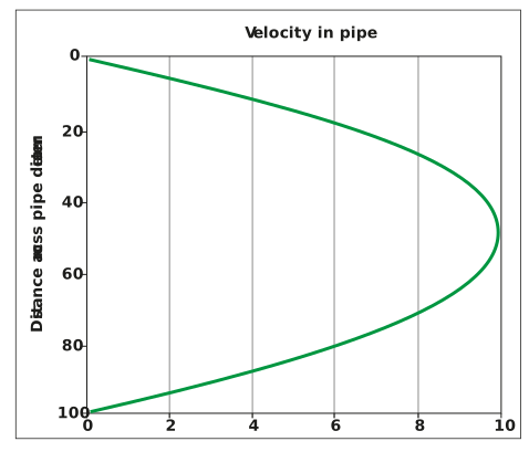
Figure: Laminar flow velocity profile across a 100 mm diameter pipe

Things to take note of in this profile include the following:

• The velocity of the fluid next to the wall (at 0 and 100 mm across the pipe) approaches zero.

• The velocity increases as we move away from the wall until the velocity reaches a maximum at the pipe centreline. (This should not be a surprise. Think of a river’s velocity as you wade across it).

• The shape of the velocity profile can be described mathematically as a parabola. Do not worry about the maths behind this!

Parabolas and parabolic shapes are all around us. For example:

• The path of a bullet fired from a gun

• A parabolic reflector in a car headlight used to focus light into a beam

• A parabolic collector for a satellite dish

The mathematical description of a parabola allows a relationship to be developed between the mean velocity and the maximum velocity; the latter measured at the centreline of the pipe. This relationship is as follows:

Where u_max is the maximum velocity and u_mean is the mean velocity.

Laminar flow is considered to be present for Reynolds numbers up to 2,100.

Let us consider the limits of Re in a worked example, based on the previous bright beer main example. 

Example:

Bright beer is flowing down a pipe of 125 mm ID. If the density and viscosity are 1,005 kg/m³ and 2 cP, respectively, what is the maximum velocity required to maintain laminar flow?

The limiting Reynolds number to maintain laminar flow is Re = 2,100. We need to find the mean velocity which corresponds to this:

Rearranging for mean velocity u:

We can see that the required maximum velocity to ensure we maintain laminar flow of the bright beer, as described, is quite low at 0.033 m/s.

Laminar flow brewery fluids

Generally, the more viscous or dense fluids are moved around a brewery under laminar flow. Examples of these would be:

• Yeast slurries

• Liquid extracts

• Boiler fuel oil

Let us summarise the key points about laminar flow.

Laminar flow:

• Smooth-flowing, calm, well-ordered stream of fluid

• Re < 2,100

•